Figure.S6.Rmd

Adding mouse homolog data

In order to do any simulation, we need to add mouse homologs to the mix. I used a modified version of the Homologene database from MGI, which only contained genes with 1-to-1 mouse-human homologs. I then will merge the tables and remove genes with no 1-to-1 mouse homolog, much like a did when calculated numbers for our analyses.

# First need to load and process the mouse MGI data
# Processed in the "biomart.finding.genes.Rmd"
homolog.table <- read.delim(file.path(file_dir,"one-one.homologs.txt"))

# Merge these tables in order to add mouse genes to dat os they can be scored
dat.merge <- unique(merge(dat, homolog.table, by.x = "hgnc_symbol", by.y = "HumanSymbol", all.x = T))

# Check for duplicated rows
summary(duplicated(dat.merge))

##    Mode   FALSE    NA's 
## logical 1308796       0

# Check number of unique SNPs queried
length(levels(dat.merge$snp))

## [1] 40213

# Remove those without mouse homologs
filtered.dat.merge <- dat.merge[!is.na(dat.merge$MouseSymbol),]

# Check number of unique SNPs again
length(levels(filtered.dat.merge$snp))

## [1] 40213

Score genes for expression

Now that I have a final dataset to work with, I can score the genes based on expression in our SN DA cluster as well as from the La Manno SN DA cluster.

# Loading in the SN expression data SNC expressed genes in our data
SN.expressed.genes <- readRDS(file = file.path(Rdata_dir, "SN.expressed.genes.rds"))

# SNC expresed genes in Linnarsson Data
lin.snc.exprs <- readRDS(file = file.path(Rdata_dir, "lin.snc.expressed.rds"))

# Scoring based on expression
filtered.dat.merge$expression <- as.factor(if_else(filtered.dat.merge$MouseSymbol %in% 
    SN.expressed.genes, 1, 0))

# Scoring based on being expressed in Lin
filtered.dat.merge$lin.exprs <- as.factor(if_else(filtered.dat.merge$MouseSymbol %in% 
    lin.snc.exprs, 1, 0))

Summarizing data

Now that every gene in every locus is scored for expression, the data needed to be summarized by locus. Data will be summarized at the level of total genes with 1:1 human:mouse homologs in the locus as well as by how many genes are expressed in each locus

# Summarizing
dat.merge.sum <- filtered.dat.merge %>%
  dplyr::group_by(snp) %>%
  dplyr::summarise(total.genes = n(),
                   exprs.genes = sum(expression == 1 | lin.exprs == 1))

## Warning: package 'bindrcpp' was built under R version 3.3.2

Figure S6A

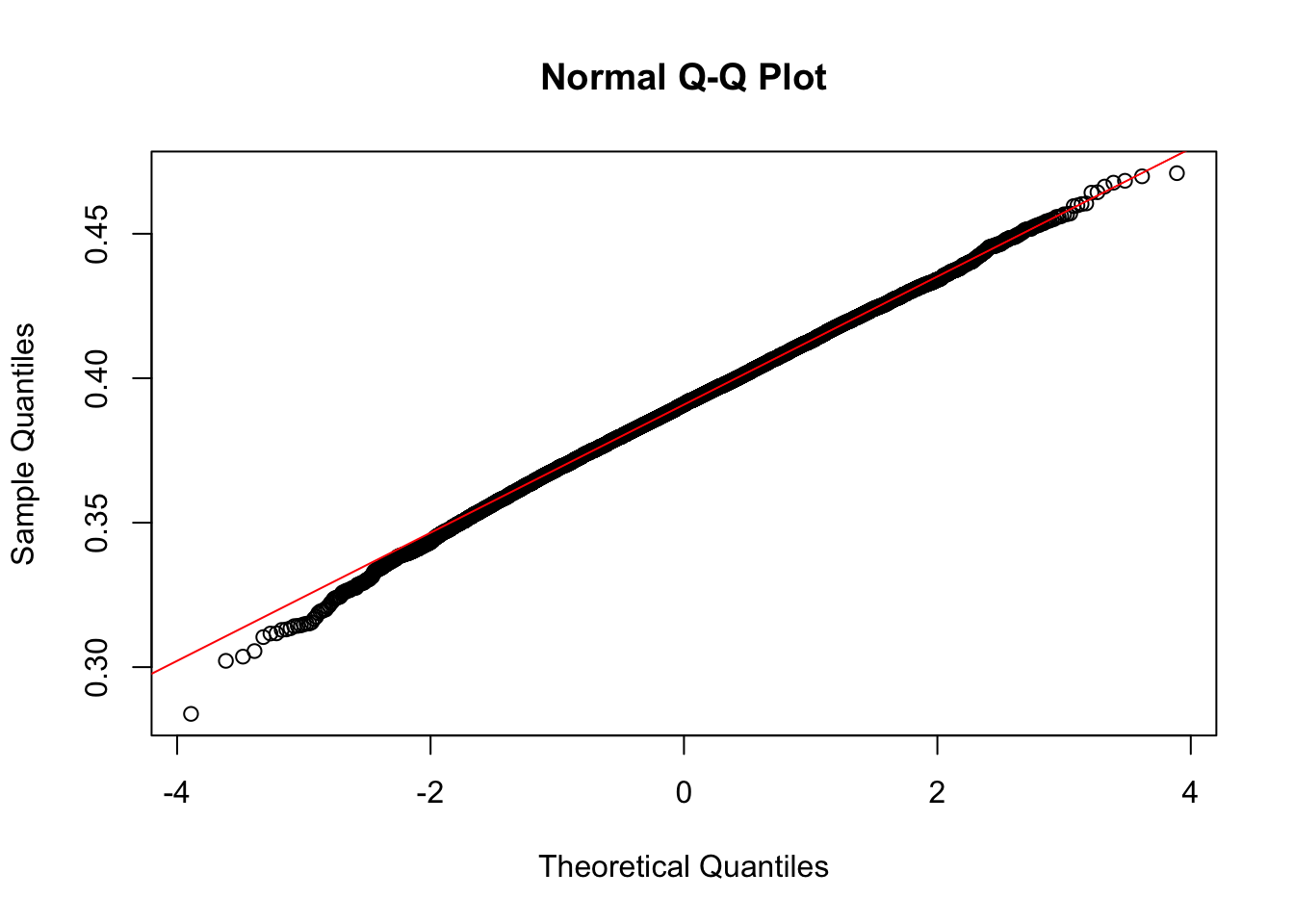
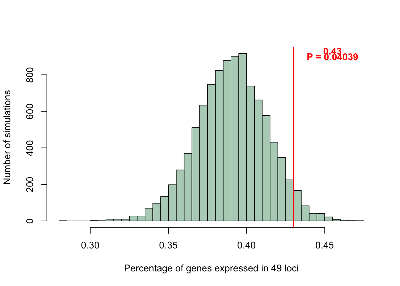
A permutation needed to be set up that would randomly sample 49 loci from the summarized dataset we have (dat.merge.sum) and then compute the frequency of genes in those randomly sampled loci that are expressed. This simulation would give us some idea as to whether the percentage of expressed genes in SN DA neurons in PD GWAS loci is similar to that of random GWAS loci. Since the data appeared to be normal, the 43% figure in our data was tested for signficance.

# Setting up blank vectors to be populated
count.freq <- c()
total.freq <- c()
exprs.freq <- c()

# Running my for loop
set.seed(24)
for(i in 1:10000){
  temp <- sample_n(dat.merge.sum,49) # sampling 49 loci
  total <- sum(temp$total.genes) # Getting total number of genes in that sampling
  total.freq <- c(total,total.freq) # Collecting that number
  exprs <- sum(temp$exprs.genes) # Getting total number of expressed genes in that sampling
  exprs.freq <- c(exprs, exprs.freq) # Collecting that number
  freq <- exprs/total # Calculating percentage of expressed genes
  count.freq <- c(freq, count.freq) # Collecting that number
  i = i + 1 # Moving the counter forward
}

# Looking at normality of the data
qqnorm(count.freq)
qqline(count.freq, col=2)

# Looking at the significance of 0.43
p.test <- pnorm(0.43,mean=mean(count.freq),sd=sd(count.freq), lower.tail = F)

p1 %<a-% {
  hist(count.freq, breaks=50,
     xlab="Percentage of genes expressed in 49 loci",
     main="",
     ylab = "Number of simulations",
     col = "#2E8B5766")
  abline(v=0.43,lwd=2,col="red")
  text(c(0.455,0.455),
      c(900,930),
      labels = c(paste0("P = ",round(p.test,5)),
                  paste0("0.43")), col = "red", font = 2)
}

pdf(file.path(file_dir,"Figure.6A.pdf"),height = 3, width = 2.5, pointsize = 8, family = 'Helvetica')
p1
dev.off()

## quartz_off_screen 
##                 2

p1

Figure S6B

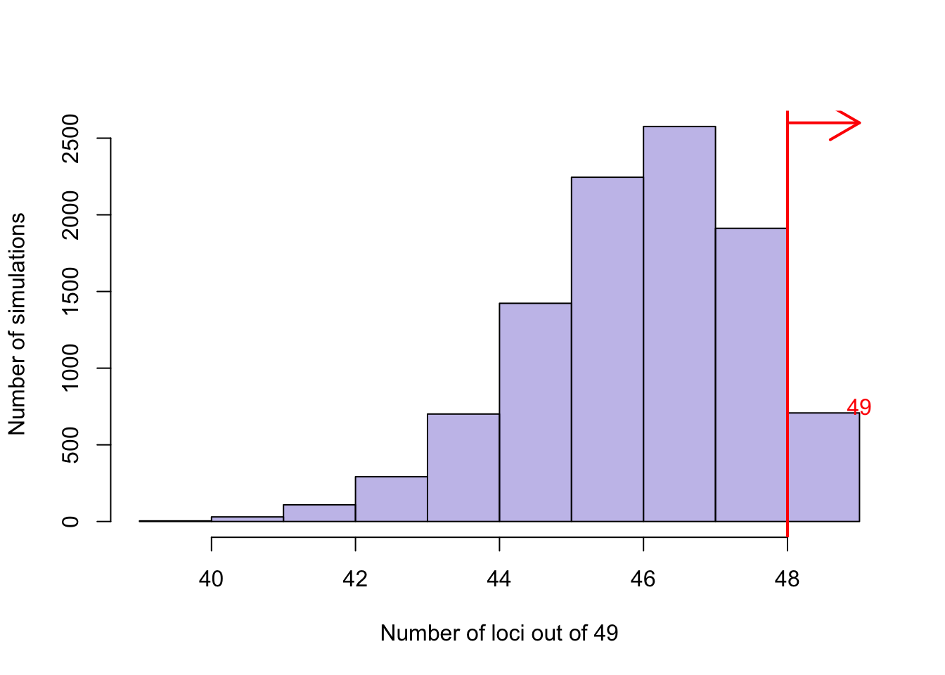
A permutation was run to see whether or not we are seeing a greater than expected number of loci with >= 1 SN expressed gene in our PD GWAS loci when compared to random GWAS loci. It does look like the majority of permutations have less than 49 loci (to the left of red line) with at least 1 gene expressed.

# Setting up blank vector to be populated
count.1 <- c()
# Running my for loop
set.seed(24)
for(i in 1:10000){
  temp <- sample_n(dat.merge.sum,49) # randomly sample 49 loci
  tf <- temp$exprs.genes >= 1 # Create a logical vector 
  num <- length(tf[tf==TRUE]) # Count loci wtih >= 1 gene expressed
  count.1 <- c(num, count.1) # Collect that number
  i = i + 1 # Move the counter
}

# Plotting
p2 %<a-% {
  hist(count.1, breaks=10,
     xlab = "Number of loci out of 49",
     ylab = "Number of simulations",
     main = "",
     col="#6A5ACD66")
  abline(v=48, lwd=2, col="red")
  text("49",col='red',y=750,x=49)
  arrows(x0=48,x1=49,y0=2600,y1=2600, col='red',lwd=2)
}

pdf(file.path(file_dir,"one.gene_loci_simulation.pdf"), height = 3, width = 2.5, pointsize = 8, family = 'Helvetica')
p2
dev.off()

## quartz_off_screen 
##                 2

p2

Figure S6C

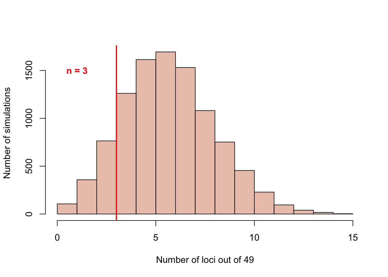
A permutation was run in order to see if the number of PD GWAS loci with only one SN DA neuron expressed gene that we find in our paper (n = 3) is different than what we would expect from 49 random GWAS loci. We see that only finding 3/49 loci wtih 1 gene expressed is actually lower than what would be expected from random loci.

# Set up blank vector
count <- c()
# Running for loop
set.seed(24)
for(i in 1:10000){
  temp <- sample_n(dat.merge.sum,49) # sampling 49 loci
  tf <- temp$exprs.genes == 1 # Making on a logical vector
  num <- length(tf[tf==TRUE]) # counting number of loci wtih exactly 1 gene expressed
  count <- c(num, count) # Collecting that number
  i = i + 1 # Move that counter!
}

p3 %<a-% {
  hist(count, breaks=20,
       xlab = "Number of loci out of 49",
       ylab = "Number of simulations",
       main = "",
       col = add.alpha("sienna3",alpha=0.4))
  abline(v=3, lwd=2, col="red")
  text("n = 3",x=1,y=1500, font = 2, col = 'red')
}

#main = "Simulation of NHGRI GWAS loci\nwith *only* 1 gene expressed in SN DA neurons"

pdf(file.path(file_dir,"only.one_simulation.pdf"), width = 3, height = 2.5, pointsize = 8, family = 'Helvetica')
p3
dev.off()

## quartz_off_screen 
##                 2

p3

Session Info

sessionInfo()

## R version 3.3.0 (2016-05-03)
## Platform: x86_64-apple-darwin13.4.0 (64-bit)
## Running under: OS X 10.11.6 (El Capitan)
## 
## locale:
## [1] en_US.UTF-8/en_US.UTF-8/en_US.UTF-8/C/en_US.UTF-8/en_US.UTF-8
## 
## attached base packages:
##  [1] grid      splines   stats4    parallel  stats     graphics  grDevices
##  [8] utils     datasets  methods   base     
## 
## other attached packages:
##  [1] bindrcpp_0.2        pryr_0.1.3          ggbiplot_0.55      
##  [4] scales_0.5.0        SC3_1.1.4           ROCR_1.0-7         
##  [7] jackstraw_1.1.1     lfa_1.2.2           tsne_0.1-3         
## [10] gridExtra_2.3       slackr_1.4.2        vegan_2.4-4        
## [13] permute_0.9-4       MASS_7.3-47         gplots_3.0.1       
## [16] RColorBrewer_1.1-2  Hmisc_4.0-3         Formula_1.2-2      
## [19] survival_2.41-3     lattice_0.20-35     Heatplus_2.18.0    
## [22] Rtsne_0.13          pheatmap_1.0.8      tidyr_0.7.1        
## [25] dplyr_0.7.4         plyr_1.8.4          heatmap.plus_1.3   
## [28] stringr_1.2.0       marray_1.50.0       limma_3.28.21      
## [31] reshape2_1.4.3      monocle_2.2.0       DDRTree_0.1.5      
## [34] irlba_2.2.1         VGAM_1.0-2          ggplot2_2.2.1      
## [37] Biobase_2.32.0      BiocGenerics_0.18.0 Matrix_1.2-11      
## 
## loaded via a namespace (and not attached):
##  [1] RSelenium_1.7.1        colorspace_1.3-2       class_7.3-14          
##  [4] rprojroot_1.2          htmlTable_1.9          corpcor_1.6.9         
##  [7] base64enc_0.1-3        mvtnorm_1.0-6          codetools_0.2-15      
## [10] doParallel_1.0.11      robustbase_0.92-7      knitr_1.17            
## [13] jsonlite_1.5           cluster_2.0.6          semver_0.2.0          
## [16] shiny_1.0.5            rrcov_1.4-3            httr_1.3.1            
## [19] backports_1.1.1        assertthat_0.2.0       lazyeval_0.2.1        
## [22] formatR_1.5            acepack_1.4.1          htmltools_0.3.6       
## [25] tools_3.3.0            igraph_1.1.2           gtable_0.2.0          
## [28] glue_1.1.1             binman_0.1.0           doRNG_1.6.6           
## [31] Rcpp_0.12.14           slam_0.1-37            gdata_2.18.0          
## [34] nlme_3.1-131           iterators_1.0.8        mime_0.5              
## [37] rngtools_1.2.4         gtools_3.5.0           WriteXLS_4.0.0        
## [40] XML_3.98-1.9           DEoptimR_1.0-8         yaml_2.1.15           
## [43] pkgmaker_0.22          rpart_4.1-11           fastICA_1.2-1         
## [46] latticeExtra_0.6-28    stringi_1.1.5          pcaPP_1.9-72          
## [49] foreach_1.4.3          e1071_1.6-8            checkmate_1.8.4       
## [52] caTools_1.17.1         rlang_0.1.6            pkgconfig_2.0.1       
## [55] matrixStats_0.52.2     bitops_1.0-6           qlcMatrix_0.9.5       
## [58] evaluate_0.10.1        purrr_0.2.4            bindr_0.1             
## [61] htmlwidgets_0.9        magrittr_1.5           R6_2.2.2              
## [64] combinat_0.0-8         wdman_0.2.2            foreign_0.8-69        
## [67] mgcv_1.8-22            nnet_7.3-12            tibble_1.3.4          
## [70] KernSmooth_2.23-15     rmarkdown_1.8          data.table_1.10.4     
## [73] HSMMSingleCell_0.106.2 digest_0.6.12          xtable_1.8-2          
## [76] httpuv_1.3.5           openssl_0.9.7          munsell_0.4.3         
## [79] registry_0.3