Cplx1 Striatum Th+ Density Analysis

Setting important directories. Also loading important libraries and custom functions for analysis.

seq_dir <- "/Volumes/PAULHOOK/sc-da-parkinsons/data"
file_dir <- "/Volumes/PAULHOOK/sc-da-parkinsons/output"
Rdata_dir <- "/Volumes/PAULHOOK/sc-da-parkinsons/data"
Script_dir <- "/Volumes/PAULHOOK/sc-da-parkinsons/code"
source(file.path(Script_dir,'init.R'))
source(file.path(Script_dir,"tools_R.r"))

#loading any special libraries
library(nlme)
library(ggpubr)
library(ggbeeswarm)
library(DT)

Loading data

First, we need to load the data from Th+ striatal quantification in WT and Cplx1 KO mice.

# Loading data
dat <- read.delim(file = file.path(Rdata_dir,"combined_quantification.txt"))
# Making sure the 'mouse' column is a factor.
dat$mouse <- as.factor(dat$mouse)

datatable(data = dat, caption = "Th+ density measurements")

Processing and initial visualization of the data

In order to analyze the data, we had to process it some first. “Blanks” which were measurements of the cortical Th+ staining in each section were removed, a unqiue identifier for each section was added and then mice were annotated as being “WT” or “KO”

#Remove 0s 'adjusted.mean' which are from the cortical measurements
dat <- dat[dat$blank == "no",]

#adding a unique section variable
dat$section.sum <- paste0(dat$mouse, ".", dat$slide, ".", dat$section)

#KO and WT
ko <- c("xif.288", "xif.291", "xif.263","bif.299", "xim.932","xim.935","xif.122","xif.145")
wt <- c("xim.636","xim.666","xif.90")

#Annotating with KO or WT
dat <- dat %>%
  mutate(condition = factor(if_else(mouse %in% ko, "KO",
               if_else(mouse %in% wt, "WT", "NA")),levels = c("WT","KO")))

## Warning: package 'bindrcpp' was built under R version 3.3.2

# Inital visualization of the data factored by condition
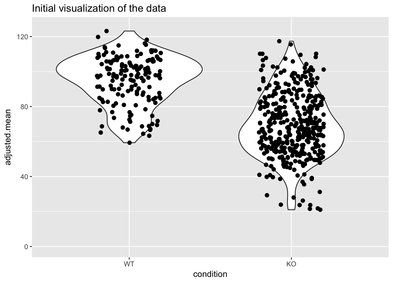
p <- ggplot(dat, aes(condition,adjusted.mean))
p + geom_violin() + geom_jitter(size = 2, width = 0.2) + ylim(c(0,125)) + ggtitle("Initial visualization of the data")

Summarizing data

We decided to summarize the data by section since they were all independently stained and measured. This way we could also preserve variation seen within each mouse brain. The data summarized by mouse showed the same outcome. We also added information about age, date IHC was performed, and sex.

# Summarizing the data based on individual section means
dat.sum <- dat %>%
  dplyr::group_by(section.sum) %>%
  dplyr::summarize(section.mean = mean(adjusted.mean))

# Add in mouse annotation column
dat.sum$mouse <- gsub("^([^.]*.[^.]*)..*$", "\\1",dat.sum$section.sum)

# Add in condition and age annotation columns
dat.sum.new <- dat.sum %>%
  mutate(condition = factor(if_else(mouse %in% ko, "KO",
               if_else(mouse %in% wt, "WT", "NA")), levels = c("WT","KO"))) %>%
  mutate(age = factor(if_else(mouse %in% c("xif.90","bif.299","xim.932","xim.935","xif.122","xif.145"), "4",
                              if_else(mouse %in% c("xim.636","xif.288","xif.291", "xif.263"), "7",
                                      if_else(mouse %in% "xim.666", "7.5", "NA"))), levels = c("4","7",
                                                                                               "7.5"))) %>%
  mutate(date = factor(if_else(mouse %in% c("xim.636","xif.288","xif.291"), "4/20/04",
                              if_else(mouse %in% "xif.263", "12/02/04",
                                      if_else(mouse %in% "bif.299", "12/09/04",
                                              if_else(mouse %in% c("xif.90","xif.122","xif.145"), "5/19/05",
                                                      if_else(mouse %in% "xim.935", "6/12/05",
                                                              if_else(mouse %in% c("xim.932","xim.666"),
                                                                      "6/17/05", "NA")))))))) %>%
  mutate(sex = factor(if_else(mouse %in% c("xim.935", "xim.932","xim.666","xim.636"),"male","female")))

Statistical Testing

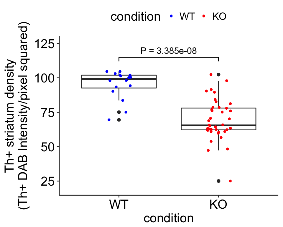
We now wanted to test to see if there is a statistcally significant difference between Th+ fiber density in the striatum between Cplx1 KO and WT littermates. We do this by performing a two sided T-test.

# First test if the variances in each condition are unequal
var <- var.test(section.mean~condition, dat.sum.new)
var

## 
##  F test to compare two variances
## 
## data:  section.mean by condition
## F = 0.52323, num df = 15, denom df = 39, p-value = 0.1765
## alternative hypothesis: true ratio of variances is not equal to 1
## 95 percent confidence interval:
##  0.2387678 1.3549478
## sample estimates:
## ratio of variances 
##          0.5232282

# Perform a two-sided t-test with equal variance
test <- t.test(section.mean~condition, dat.sum.new, alternative = "two.sided", var.equal = T, conf.level = 0.95)
test

## 
##  Two Sample t-test
## 
## data:  section.mean by condition
## t = 6.4359, df = 54, p-value = 3.385e-08
## alternative hypothesis: true difference in means is not equal to 0
## 95 percent confidence interval:
##  17.79191 33.89214
## sample estimates:
## mean in group WT mean in group KO 
##         95.01971         69.17768

Visualization

# Plot the independent section measurements by condition
set.seed(2)
p <- ggplot(dat.sum.new, aes(condition,section.mean))
final <- p + geom_boxplot() + 
  geom_point(size = 1, position = position_jitterdodge(jitter.width = 0.5), aes(color = condition)) + 
  theme_pubr() + 
  ylab("Th+ striatum density\n(Th+ DAB Intensity/pixel squared)") + 
  theme(plot.title = element_text(hjust = 0.5)) +
  scale_color_manual(values = c("blue","red")) + 
  theme(text = element_text(size=16)) + ylim(c(20,125)) +
  annotate("text", x=1.5,y=120,label=paste0("P = ",round(test$p.value,11)),size=4) +
  annotate("segment", x = 1, xend = 2, y = 115, yend = 115, lwd=0.5) +
  annotate("segment", x=1, xend=1,y=112,yend=115,lwd=0.5) +
  annotate("segment", x=2, xend=2,y=112,yend=115,lwd=0.5)

pdf(file = file.path(file_dir,"Figure.5E.pdf"), height = 4, width = 5)
final
dev.off()

## quartz_off_screen 
##                 2

final