Figure 1
Paul Hook
Last update: 2018-01-18
Code version: 5996c19850dc5fc65723f30bc33ab1c8d083a7e6
Setting important directories. Also loading important libraries and custom functions for analysis.
seq_dir <- "/Volumes/PAULHOOK/sc-da-parkinsons/data"
file_dir <- "/Volumes/PAULHOOK/sc-da-parkinsons/output"
Rdata_dir <- "/Volumes/PAULHOOK/sc-da-parkinsons/data"
Script_dir <- "/Volumes/PAULHOOK/sc-da-parkinsons/code"
source(file.path(Script_dir,'init.R'))
source(file.path(Script_dir,"tools_R.r"))

#loading any special libraries
library(readr)
library(cowplot)
Loading the cds data needed to produce figures
In order to produce the figures seen in Figure 1, we needed to load:
- The final valid cell dataset (dat.filter.final.Rds)
- The PCA results using genes with a high biological variance in the entire dataset
- GSEA results for PC1
dat.filter <- readRDS(file.path(Rdata_dir,"dat.filter.final.Rds"))
dat.filter.BCV.pca <- readRDS(file.path(Rdata_dir, "dat.filter.BCV.pca"))
path_to_sheets <- file.path(file_dir, "PC1.all.cells.3_27_17.GseaPreranked.1490670535140")
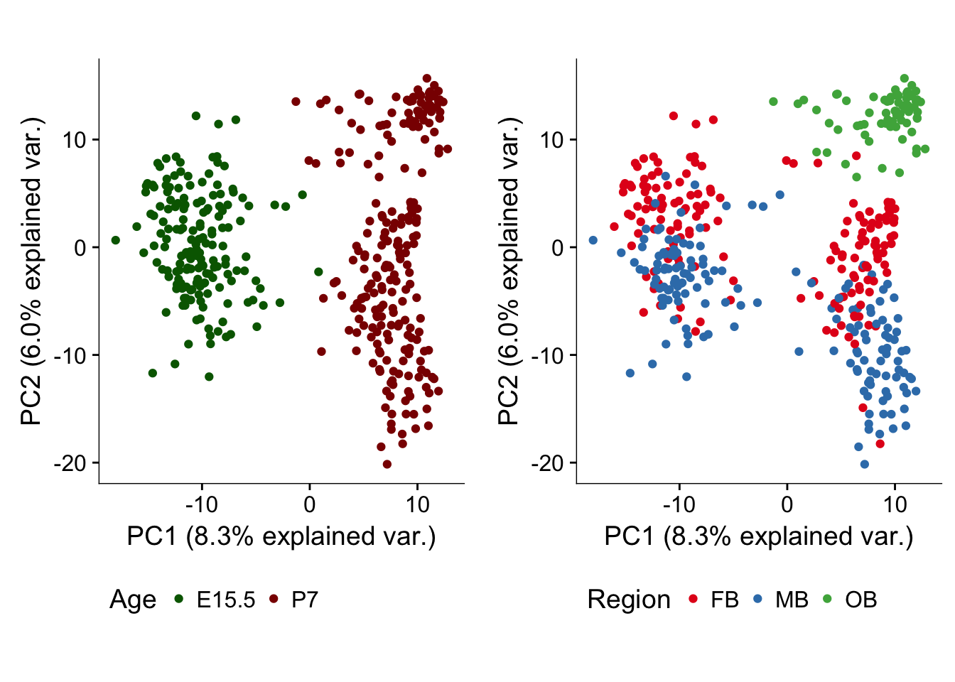
Figure 1B
This panel shows the results from running principle component analysis (PCA) using genes with a high biological variance in all the valid cells in our dataset. One part of the panel will show the cells colored by timepoint, the other part of the panel will show the cells colored by regional identity.
p <- ggbiplot(dat.filter.BCV.pca,choices=c(1,2),scale=0,groups=pData(dat.filter)$age,ellipse=F,var.axes=F) + scale_color_manual(values=c("darkgreen","darkred")) + monocle:::monocle_theme_opts() + theme(legend.position = "bottom",axis.line = element_line(colour = "black")) + coord_fixed(ratio = 1) + labs(color = "Age")

q <- ggbiplot(dat.filter.BCV.pca,choices=c(1,2),scale=0,groups=pData(dat.filter)$region,ellipse=F,var.axes=F) + scale_color_brewer(palette="Set1") + monocle:::monocle_theme_opts() + theme(legend.position = "bottom",axis.line = element_line(colour = "black")) + coord_fixed(ratio = 1) + labs(color = "Region")

pdf(file = file.path(file_dir, "Figure.1B.pdf"), width = 4, height = 4)
p
q
dev.off()
## quartz_off_screen
## 2plot_grid(p,q,ncol=2)
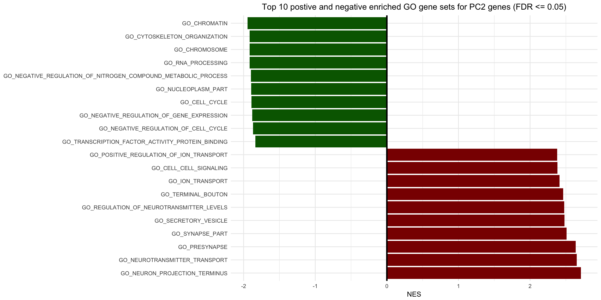
Figure 1C
This script is meant to take the GSEA output Excel sheets and make a double sided barplot displaying the enrichment scores of significant gene sets
# We now need to "construct" the file name of the of the Excel files that contain the GSEA output that we want. Those are normally named "gsea_report_for_na_" + "pos_" or "neg_" + GSEA number + ".xls"

# The first step is to extract the GSEA number from the directory file path
path_unlisted <- unlist(strsplit(path_to_sheets, split = "/"))
dir_name <- path_unlisted[length(path_unlisted)]
dir_name_unlisted <- unlist(strsplit(dir_name, split = ".", fixed = T))
gsea_number <- dir_name_unlisted[length(dir_name_unlisted)]

# Next, I want to save the beginning of the file names as  variable I can use later
gsea_preamble <- "gsea_report_for_na"

# Now I can construct the Excel file names for the positive and negative results
gsea_pos <- paste0(gsea_preamble, "_", "pos", "_", gsea_number, ".xls")
gsea_neg <- paste0(gsea_preamble, "_", "neg", "_", gsea_number, ".xls")

# I want to first set the path to each of the Excel sheets, then make sure that the files exist in the paths that I expect them to be in
pos.file <- file.path(path_to_sheets, gsea_pos)
neg.file <- file.path(path_to_sheets, gsea_neg)
#file.exists(pos.file)
#file.exists(neg.file)

# I want to first load the data now that I have the path
pos.set <- read_delim(file = file.path(path_to_sheets, gsea_pos), delim = "\t")
## Warning: Missing column names filled in: 'X12' [12]## Parsed with column specification:
## cols(
## NAME = col_character(),
## `GS<br> follow link to MSigDB` = col_character(),
## `GS DETAILS` = col_character(),
## SIZE = col_integer(),
## ES = col_double(),
## NES = col_double(),
## `NOM p-val` = col_double(),
## `FDR q-val` = col_double(),
## `FWER p-val` = col_double(),
## `RANK AT MAX` = col_integer(),
## `LEADING EDGE` = col_character(),
## X12 = col_character()
## )# Then I want to clean up the data so that I only retain the data I want. I will do this using the dplyr package and protocol
pos.set <- pos.set %>%
dplyr::select(NAME,SIZE, ES, NES, `NOM p-val`, `FDR q-val`, `FWER p-val`)
# Had to rename outside of the pipe because for some reason I could not rename some of the columns
names(pos.set) <- c("Name","Size","ES","NES","NOM p.val","FDR q.val", "FWER p.val")
# Going back in to the pipe now, I only want gene sets with an FDR <= 0.05 and I only want the top 10. I only need to "head" the top 10 because the Excel sheets are already ordered with lowest p-value on top
pos.set <- pos.set %>%
filter(`FDR q.val` <= 0.05) %>%
head(10)## Warning: package 'bindrcpp' was built under R version 3.3.2# I want to first load the data now that I have the path
neg.set <- read_delim(file = file.path(path_to_sheets, gsea_neg), delim = "\t")## Warning: Missing column names filled in: 'X12' [12]## Parsed with column specification:
## cols(
## NAME = col_character(),
## `GS<br> follow link to MSigDB` = col_character(),
## `GS DETAILS` = col_character(),
## SIZE = col_integer(),
## ES = col_double(),
## NES = col_double(),
## `NOM p-val` = col_double(),
## `FDR q-val` = col_double(),
## `FWER p-val` = col_double(),
## `RANK AT MAX` = col_integer(),
## `LEADING EDGE` = col_character(),
## X12 = col_character()
## )# Then I want to clean up the data so that I only retain the data I want. I will do this using the dplyr package and protocol
neg.set <- neg.set %>%
dplyr::select(NAME,SIZE, ES, NES, `NOM p-val`, `FDR q-val`, `FWER p-val`)
# Had to rename outside of the pipe because for some reason I could not rename some of the columns
names(neg.set) <- c("Name","Size","ES","NES","NOM p.val","FDR q.val", "FWER p.val")
# Going back in to the pipe now, I only want gene sets with an FDR <= 0.05 and I only want the top 10. I only need to "head" the top 10 because the Excel sheets are already ordered with lowest p-value on top
neg.set <- neg.set %>%
filter(`FDR q.val` <= 0.05) %>%
head(10)
# I then want to combine both the positive and negative data sets and give the postitive and negative NES values colors for plotting.
all.set <- rbind(neg.set, pos.set) %>%
mutate(NES_direction = if_else(NES > 0, "darkred", "darkgreen"))
# Making the plot
b <- ggplot(all.set) + geom_bar(aes(x=reorder(Name, -NES),y=NES,fill=NES_direction),stat='identity') + coord_flip() + xlab("GO Gene Set") + theme_minimal(base_size = 10) + scale_fill_identity() + geom_hline(yintercept = 0, size = 1) + theme(axis.title.y = element_blank(), plot.title = element_text(hjust = 0.5)) + ggtitle("Top 10 postive and negative enriched GO gene sets for PC2 genes (FDR <= 0.05)")
# Write the plot out to a pdf
pdf(file = file.path(file_dir,"Figure.1C.pdf"), width = 10, height = 6)
b
dev.off()## quartz_off_screen
## 2b
Figures 1D and 1E
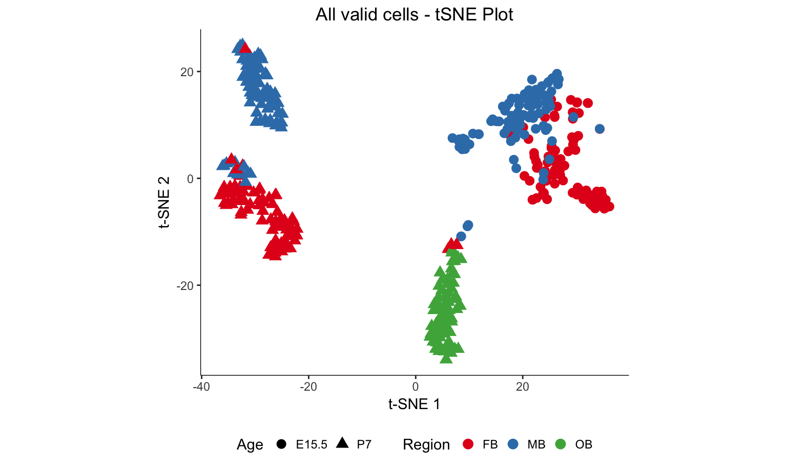
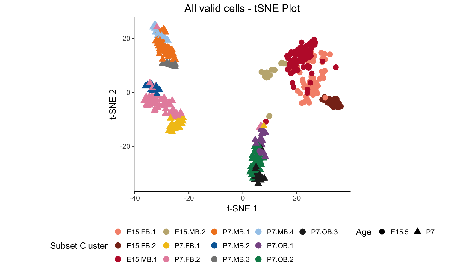
The following script was used to produce the t-SNE plots of all the cells that passed QC. One plot (Figure 1D) will show the plot colored by brain region and one plot (Figure 1E) will show the plot colored by subset clusters identified through iterative analysis.
# Setting up colors
library(pals)
#Random shuffling of 13 colors to get a combination I like
#color.sample <- sample(kelly(22)[c(2:12,13,18)])

#Setting the order of a good looking set of hex codes
color <- c("#F6937A","#882F1C","#BF1F36","#C2B280","#F2C318","#E790AC","#F18421","#0168A5","#848483","#A4CAEB","#885793","#008957","#222222")

# tSNE colored by region
r <- myTSNEPlotAlpha(dat.filter,color="region", shape="age") + scale_color_brewer(palette="Set1", name = "Region") + ggtitle("All valid cells - tSNE Plot") + xlab("t-SNE 1") + ylab("t-SNE 2") + theme(legend.position = "bottom",axis.line = element_line(colour = "black")) + theme(plot.title = element_text(hjust = 0.5)) + coord_fixed(ratio = 1) + scale_shape(name = "Age")

# tSNE colored by regional subsets
s <- myTSNEPlotAlpha(dat.filter,color="subset.cluster", shape="age") + scale_color_manual(values = color, name = "Subset Cluster") + ggtitle("All valid cells - tSNE Plot") + xlab("t-SNE 1") + ylab("t-SNE 2") + theme(legend.position = "bottom",axis.line = element_line(colour = "black")) + theme(plot.title = element_text(hjust = 0.5)) + coord_fixed(ratio = 1) + scale_shape(name = "Age")

pdf(file = file.path(file_dir, "Figure.1D-1E.pdf"), width = 8, height = 8)
r
s
dev.off()
## quartz_off_screen
## 2r
s
Session Info
sessionInfo()## R version 3.3.0 (2016-05-03)
## Platform: x86_64-apple-darwin13.4.0 (64-bit)
## Running under: OS X 10.11.6 (El Capitan)
##
## locale:
## [1] en_US.UTF-8/en_US.UTF-8/en_US.UTF-8/C/en_US.UTF-8/en_US.UTF-8
##
## attached base packages:
## [1] grid splines stats4 parallel stats graphics grDevices
## [8] utils datasets methods base
##
## other attached packages:
## [1] pals_1.4 maps_3.2.0 bindrcpp_0.2
## [4] cowplot_0.9.2 readr_1.1.1 ggbiplot_0.55
## [7] scales_0.5.0 SC3_1.1.4 ROCR_1.0-7
## [10] jackstraw_1.1.1 lfa_1.2.2 tsne_0.1-3
## [13] gridExtra_2.3 slackr_1.4.2 vegan_2.4-4
## [16] permute_0.9-4 MASS_7.3-47 gplots_3.0.1
## [19] RColorBrewer_1.1-2 Hmisc_4.0-3 Formula_1.2-2
## [22] survival_2.41-3 lattice_0.20-35 Heatplus_2.18.0
## [25] Rtsne_0.13 pheatmap_1.0.8 tidyr_0.7.1
## [28] dplyr_0.7.4 plyr_1.8.4 heatmap.plus_1.3
## [31] stringr_1.2.0 marray_1.50.0 limma_3.28.21
## [34] reshape2_1.4.3 monocle_2.2.0 DDRTree_0.1.5
## [37] irlba_2.2.1 VGAM_1.0-2 ggplot2_2.2.1
## [40] Biobase_2.32.0 BiocGenerics_0.18.0 Matrix_1.2-11
##
## loaded via a namespace (and not attached):
## [1] RSelenium_1.7.1 colorspace_1.3-2 class_7.3-14
## [4] rprojroot_1.2 htmlTable_1.9 corpcor_1.6.9
## [7] base64enc_0.1-3 dichromat_2.0-0 mvtnorm_1.0-6
## [10] codetools_0.2-15 doParallel_1.0.11 robustbase_0.92-7
## [13] knitr_1.17 jsonlite_1.5 cluster_2.0.6
## [16] semver_0.2.0 shiny_1.0.5 mapproj_1.2-5
## [19] rrcov_1.4-3 httr_1.3.1 backports_1.1.1
## [22] assertthat_0.2.0 lazyeval_0.2.1 acepack_1.4.1
## [25] htmltools_0.3.6 tools_3.3.0 igraph_1.1.2
## [28] gtable_0.2.0 glue_1.1.1 binman_0.1.0
## [31] doRNG_1.6.6 Rcpp_0.12.14 slam_0.1-37
## [34] gdata_2.18.0 nlme_3.1-131 iterators_1.0.8
## [37] mime_0.5 rngtools_1.2.4 gtools_3.5.0
## [40] WriteXLS_4.0.0 XML_3.98-1.9 DEoptimR_1.0-8
## [43] hms_0.3 yaml_2.1.15 pkgmaker_0.22
## [46] rpart_4.1-11 fastICA_1.2-1 latticeExtra_0.6-28
## [49] stringi_1.1.5 pcaPP_1.9-72 foreach_1.4.3
## [52] e1071_1.6-8 checkmate_1.8.4 caTools_1.17.1
## [55] rlang_0.1.6 pkgconfig_2.0.1 matrixStats_0.52.2
## [58] bitops_1.0-6 rgl_0.98.1 qlcMatrix_0.9.5
## [61] evaluate_0.10.1 purrr_0.2.4 bindr_0.1
## [64] labeling_0.3 htmlwidgets_0.9 magrittr_1.5
## [67] R6_2.2.2 combinat_0.0-8 wdman_0.2.2
## [70] foreign_0.8-69 mgcv_1.8-22 nnet_7.3-12
## [73] tibble_1.3.4 KernSmooth_2.23-15 rmarkdown_1.8
## [76] data.table_1.10.4 HSMMSingleCell_0.106.2 digest_0.6.12
## [79] xtable_1.8-2 httpuv_1.3.5 openssl_0.9.7
## [82] munsell_0.4.3 registry_0.3This R Markdown site was created with workflowr